How to Optimize a Deep Learning Model for faster Inference?
Is there a way to optimize a Deep Learning model for inference? What are the processes? Is it doable easily? Or only an expert secret?
In Deep Learning, an inference is the forward propagation process that, given an input, gets the output.
For example, the classification of a 3D Point Cloud can determine the class, and the regression can retrieve the Bounding Box coordinates of obstacles in an image.

Knowing the inference time in advance can help you design a model that will perform better, and be optimized for inference.
For example, we can replace a standard convolution with a separable convolution, reducing the number of computations. We can also prune, quantize, or freeze a model.
These optimization techniques can save seconds in inference time, and drastically change the output.
Here's the general process that we'll look at in this article.
- How to calculate the inference time of a model?
- FLOPs, FLOPS, and MACs
- Calculating the FLOPs of a model
- Calculating the inference time
- How to optimize a model for better performance?
- Reducing the Number of Operations
- Reducing the Model Size
How to calculate the inference time of a model?
In order to understand how to optimize a Neural Network, we must have a metric. That metric will be the inference time.
The inference time is how long is takes for a forward propagation. To get the number of Frames per Second, we divide 1/inference time.
In order to measure this time, we must understand 3 ideas: FLOPs, FLOPS, and MACs.
FLOPs
To measure inference time for a model, we can calculate the total number of computations the model will have to perform.
This is where we mention the term FLOP, or Floating Point Operation.
This could be an addition, subtraction, division, multiplication, or any other operation that involves a floating point value.
The FLOPs will give us the complexity of our model.
FLOPS
The second thing is the FLOPS, with a capital S.
FLOPS are the Floating Point Operations per Second. This is a rate that tells us how good is our hardware.
The more operations per second we can do, the faster the inference will be.
MACs
The final thing to consider is the MACs, standing for Multiply-Accumulate Computations.
A MAC is an operation that does an addition and a multiplication, so 2 operations.
In a neural network, addition and multiplications happen every time.
Layeroutput=W1∗A1+W2∗A2+...+Wn∗An
As a rule, we consider 1 MAC = 2 FLOPs.
Now that we know this, we understand the general idea:
- We want a low number of FLOPs in our model, but keeping it complex enough to be good.
- We want a high number of FLOPS in our hardware.
- Our role will be to optimize the Deep Learning models to have a low number of FLOPs.
Calculating the FLOPs in a Model
Let's take the following model that performs a classification on the MNIST dataset.
- The Input Image is of size 28x28x1 (grayscale)
- We run 2 Convolutions of 5 kernels of size (3x3)
- We run a Fully Connected Layer of 128 Neurons
- We finish with a Fully Connected Layer of 10 Neurons: 1 per digit.
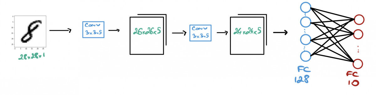
our deep learning model for MNIST classification
Each layer of this model will perform some operations, that will add up some FLOPs.
➡️ For a refresher on CNNs, you can check this cheatsheet.
To calculate the FLOPs in a model, here are the rules:
- Convolutions - FLOPs = 2x Number of Kernel x Kernel Shape x Output Shape
- Fully Connected Layers - FLOPs = 2x Input Size x Output Size
These formulas are actually made to calculate the number of MACs. The FLOPs are retrieved with the 2x at the beginning.
- Pooling Layers - FLOPs = Height x Depth x Width of an image
- With a stride, FLOPs = (Height / Stride) x Depth x (Width / Stride) of an image
- As a reminder, the output shape of a convolutional layer is Output = (Input Shape - Kernel Shape) + 1
Let's calculate this with the relationship in mind:
First Convolution - 2x5x(3x3)x26x26 = 60,840 FLOPs
Second Convolution -2x5x(3x3x5)x24x24 = 259,200 FLOPs
First FC Layer - 2x(24x24x5)x128 = 737,280 FLOPs
Second FC Layer - 2x128x10 = 2,560 FLOPs
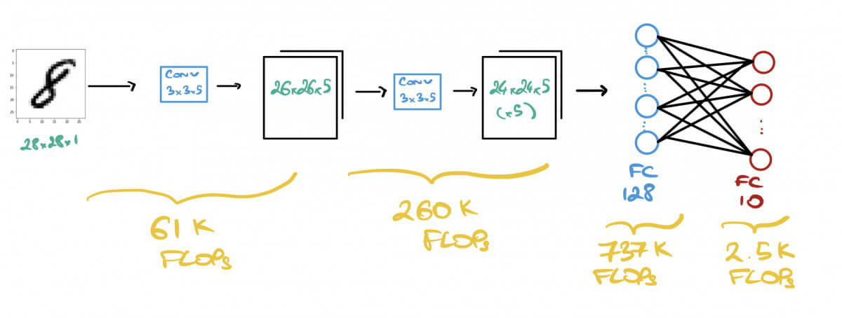
👉 The model will do FLOPs = 60,840 + 259,200 + 737,280 + 2,560 = 1,060,400 operations
Calculating the Inference Time
Say we have a CPU that performs 1 GFLOPS.
The inference time will be FLOPs/FLOPS = (1,060,400)/(1,000,000,000) = 0,001 s or 1ms.
Calculating the inference time is simple, if we have the FLOPS...
The FLOPS can be retrieved by understanding what is our processor.
The more powerful the processor, the bigger this number.
Let's now see the second part: Optimization.
How to optimize a model for better performance?
In the first part, we talked about calculating the inference time.
It means that given a Deep Learning model and a hardware, I can compute how much time it will take for a forward propagation.
Now, let's see how to optimize a deep learning model for inference.
✅ That can be very useful every day, for example when deploying, or simply when running a model.
✌🏼 At the end of this blog post, I'll give you the link to a MindMap on Deep Learning Optimization.
We have 2 main ways to optimize a neural network:
Reducing the Number of Operations
When we reduce the number of operations, we are replacing some operations with others that are more efficient.
Here, let me cite 3 operations that can work:
- Pooling
- Separable Convolutions
- Model Pruning
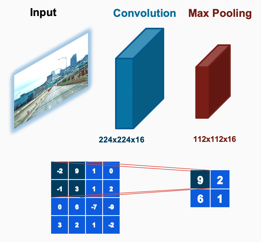
Pooling
Let's start with Pooling. If you took Deep Learning courses, you probably already know about Max Pooling or Average Pooling. These operations are part of those that reduce the number of operations.
Pooling layers are subsampling layers that reduce the amount of data or parameters being passed from one layer to another.
Pooling Layers are generally used after a convolution, to retain spatial information, while reducing the number of parameters.
Separable Convolutions
Pooling is great, but when calculating the number of FLOPs, it's still expensive.
A separable convolution is a convolutional layer that divides the standard convolutional layer into two layers: a depthwise convolution and a pointwise convolution.
- A depthwise convolution is a normal convolution, but we don't change the depth. We're therefore reducing the number of FLOPs.
- A pointwise convolution is a 1x1 convolution. Each kernel iterate over each pixel in the image.
➡️ By doing so, the number of FLOPs or operations required to run the model is reduced. Let's see on our previous example how that reduces the number of FLOPs.
The following is a separable convolution, a depthwise, followed by a pointwise:

The total number of FLOPs is 318K + 415K, or approximately 734k floating point operations.
Now, let's see the equivalent 2D convolution:

We have over 20 Million operations.
With a 1 Giga FLOPS harware, that operation alone would take 0.2s.
Separable Convolutions can drastically reduce the number of operations. We have 20M vs 734k operations, or over 20 times less when using these operations. That's almost a 0.2s difference per inference.
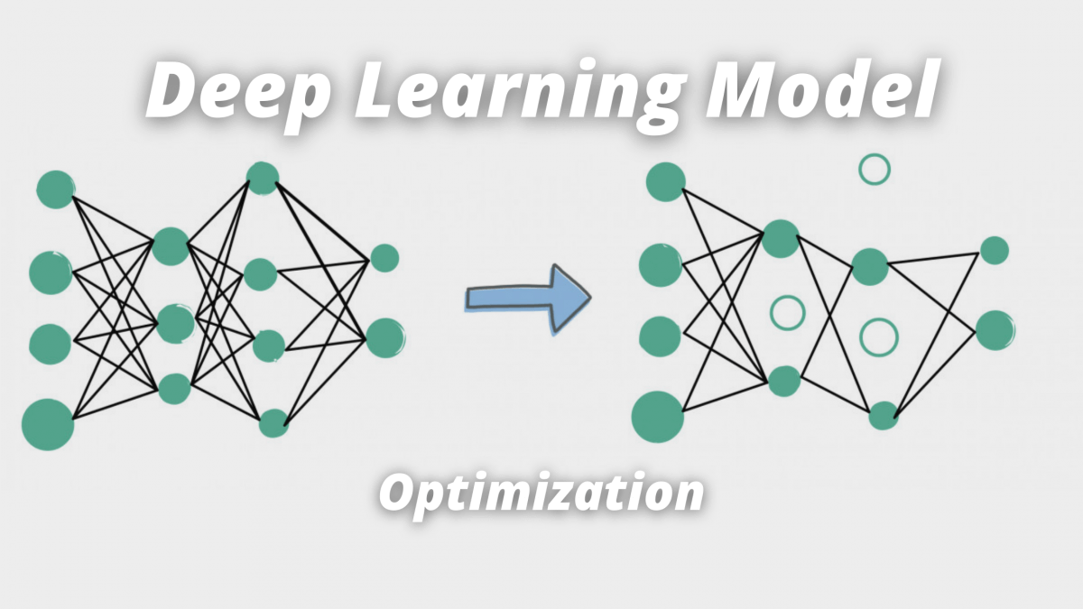
Model Pruning
Finally, let's see something called Pruning.
Pruning is a model compression technique where redundant network parameters are removed while trying to preserve the original accuracy (or other metric) of the network.
To achieve that technique, we first identify the ranks that matter, the most, and then remove those that are redundant.
To do so, we either remove the neuron, by setting the connections to it to 0, or by setting the weight to 0.

model pruningWe just saw 3 powerful techniques to optimize a Deep Neural Network by reducing the number of operations.
➡️ Please note that these can be implemented easily, with one line of code.
Now, let's see how to reduce the size of a model.
Reducing the Model Size
When we reduce the model size, we benefit of several advantages, such as faster loading, less size in storage, faster compilation, ...
We have 3 ways of reducing the size of a model:
- Quantization
- Knowledge Distillation
- Weight Sharing
Quantization
Let's start with Model Quantization, which is a compression process.
Quantization is the process of mapping values from a larger set to a smaller one. In other words, we reduce large continuous numbers and replace them with smaller continuous numbers, or even integers.
➡️ If a weight is 2.87950387409, I'll map it to 2.9 (it's not exactly this going on, but it's just an image).
We are actually changing precision.
A few things to note on Quantization:
- Quantization can be done on weights, and on activations.
- These both reduces memory and complexity of computations.
- In general, we'll use this to normalize weights, or change the range.
ex: converting weights between -3 and +5 to 0-255 range.
Weight Sharing
Quantization belongs to a family called Compression.
Weight Sharing is another technique in which we share the weights between neurons, so we have less of them to store.
👉 The K-Means algorithm can do something like this.
Knowledge Distillation
Imagine the number of things I had to go through to write this article.
I'm only sharing what matters the most, so you can focus on the essential.
➡️ That's knowledge distillation.
Knowledge distillation is a method where we try to transfer the knowledge learned by a large, accurate model (the teacher model) to a smaller and computationally less expensive model (the student model).
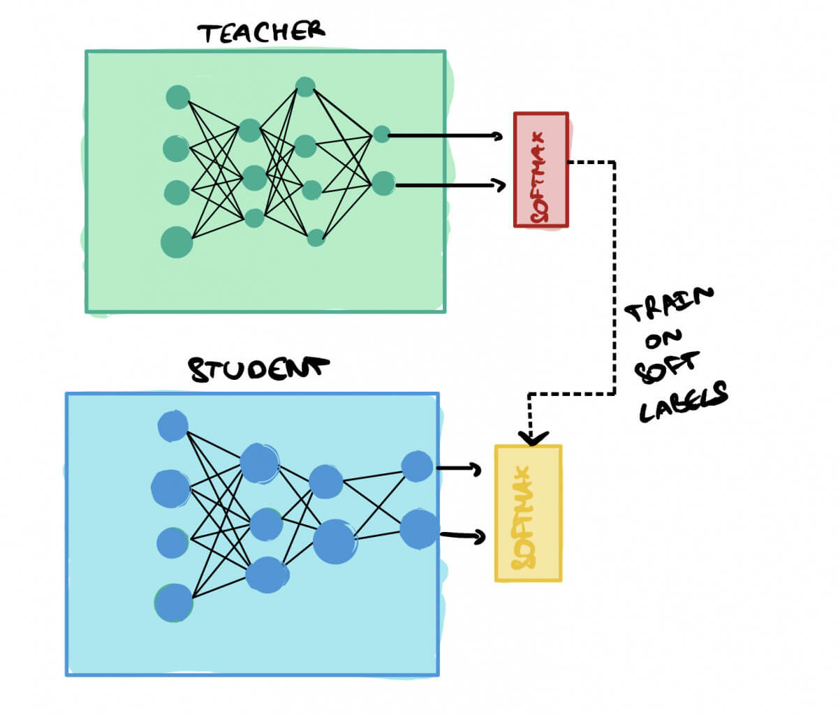
The student is trained using "soft labels", this means that, for a classification model, we'll use the softmax values.
➡️ If I have "Cat: 0.9", "Dog: 0.2", I won't switch to [1,0].
The students will be taught on the softmax.
Some results on Knowledge Distillation:

Congratulations on following this article, you now know much more about Deep Learning Optimization.
To summarize this, I have created the best (and only) mindmap on Deep Learning optimization.
From calculating the inference time, to listing the approaches for optimization we discussed. It's available for free (for now) when you join my daily emails! If you aren't aware of the Daily Emails yet, I invite you to give your email below! The Daily Emails is a free daily training that I run on AI, Computer Vision, and Self-Driving Cars, and that will help you break into the cutting-edge world.
➡️ Get your MindMap on this link .