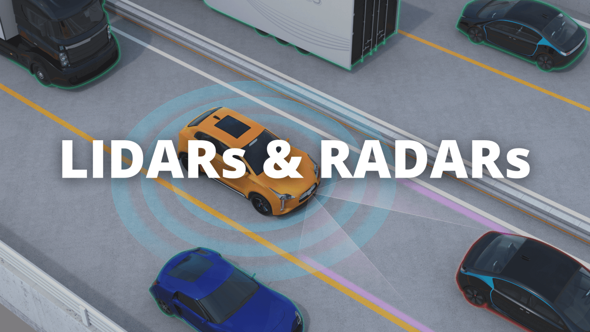
Sensor Fusion - LiDARs & RADARs in Self-Driving Cars
In this article, we'll take a deep dive into Sensor Fusion between LiDARs and RADARs. These two sensors are heavily used in autonomous driving and many other robotics applications. We'll start with a short intro on both sensors, and then move to the fusion algorithm we use, and its specificities.
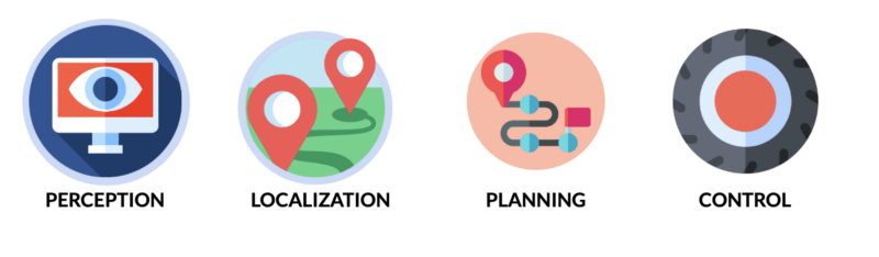
What is Sensor Fusion, by the way? In the Perception module, which is about seeing the environment (road lines, traffic signs, buildings, pedestrians, ...), we need to use multiple sensors. This can either add redundancy, certainty, or to take advantage of using multiple sensors and create multiple use-cases. This creates a field we call Sensor Fusion.
For example, using a camera allows us to see the colors of traffic lights. It's a perfect tool for classification, lane line detection, ... Using a LiDAR is great for SLAM (Simultaneous Localization And Mapping), and for depth estimation -- ie estimating the exact distance of any object. Finally, a RADAR has a specific technology that can measure velocities of objects, and give you a speed ticket!
In this article, we'll learn to fuse a LiDAR and a RADAR, and thus take advantage of the LiDARs technology to estimate distances and see a world in 3D, and the RADAR's ability to estimate velocities.
👉 If you're interested in the fusion between a LiDAR and a Camera, I'm covering it in this article .
👉 If you're interested in getting a short intro to Sensor Fusion, it's here .
Sensor Data for LiDAR RADAR Fusion
Before we consider any sensor fusion task, we must do two things:
- Pick multiple sensors to merge - and define a clear goal.
- Study both sensors to define "how" you'll fuse them.
Let's take a minute and review the different sensors...
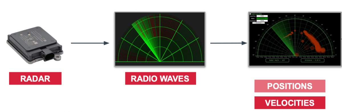
RADAR (Radio Detection and Ranging)
A RADAR emits radio waves to detect objects within a range of several meters (~150). Radars have been in our cars for years to detect vehicles in blind spots and to avoid collisions.
Unlike other sensors that calculate the difference in position between two measurements, the radar uses the Doppler effect by measuring the change in the next wave frequency if the vehicle moves towards us or moves away. This is called radial velocity.
The radar can directly estimate a speed .
Because of that, they also show better results on moving objects than on static objects.
It has a low resolution, it allows to know the position and speed of a detected object. On the other hand, it will struggle to determine "what" is the object being sensed.
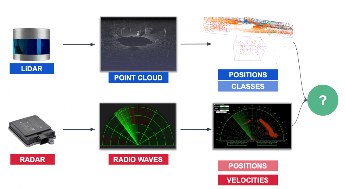
LiDAR (Light Detection and Ranging)
The LiDAR uses infrared sensors to determine the distance to an object. A rotating system makes it possible to send waves and to measure the time taken for this wave to come back to it. This makes it possible to generate a points cloud of the environment around the sensor. It can generate about 2 million points per second. A point cloud giving different 3D shapes, it is possible to make the classification of objects thanks to a Lidar, as I'm teaching in this course .

It has a good range (100 to 300 m), and can accurately estimate the position of objects around it. Itssize is however cumbersome, and it can be seen as some people as a crutch. Not mentioned, its price (1,000-50,000$) has been for years very high, andstill remains farabovethan the average price of a camera (500)oraRADAR(300) or a RADAR (300).
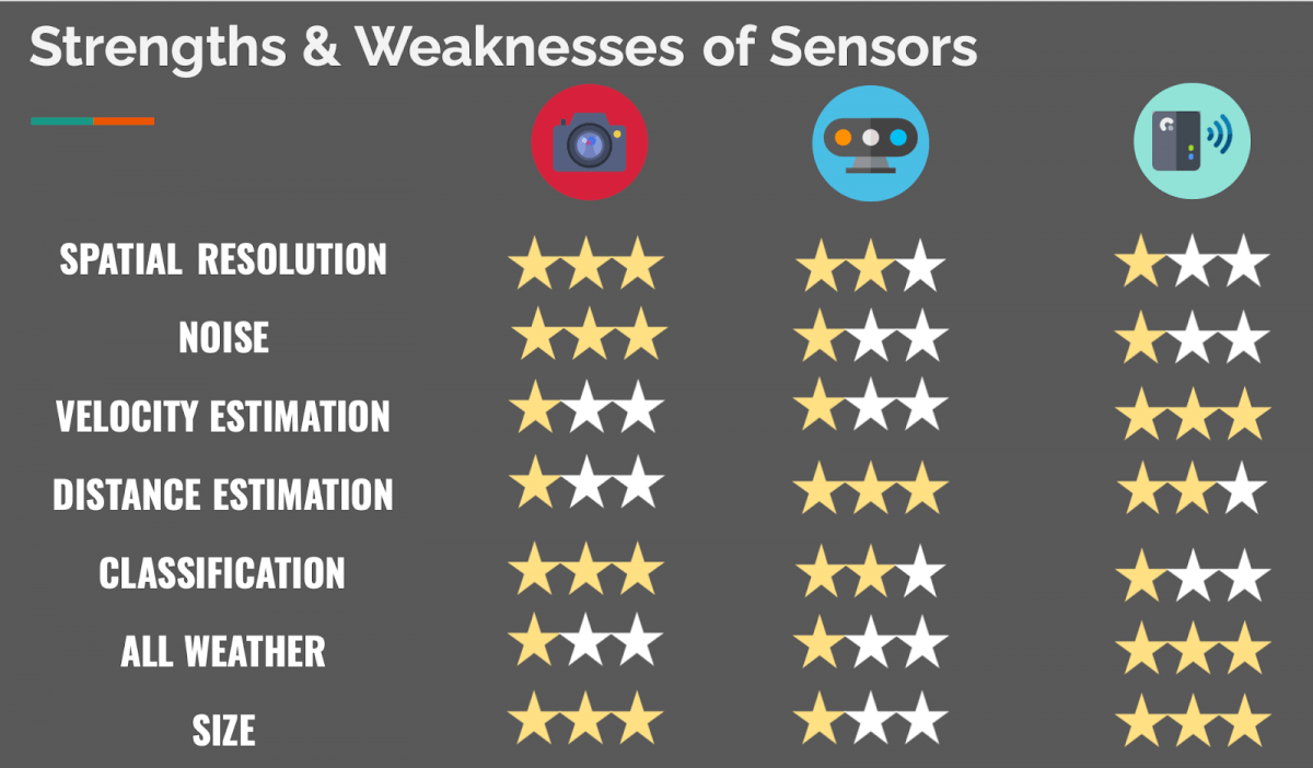
Strenght & Weaknesses of Sensors
Here are the strenghts and weaknesses of each sensor: cameras, LiDARs, and RADARs
We now know have a good idea of RADARs and LiDARS. Let's see how to fuse them!
What type of Data Fusion is used?
As I explain in this article on Sensor Fusion, we have 3 types of sensor fusion classifications:
- Low-Level Sensor Fusion - Fusing the RAW Data
- Mid-Level Sensor Fusion - Fusing the Objects
- High-Level Sensor Fusion - Fusing the Objects & their positions in time (tracking)
In my LiDAR/Camera Fusion article , I'm showing how sensor fusion works in the early level mode; fusing point clouds and pixels, and the late level mode; fusing bounding boxes and results.
In this article, we're going to focus on Mid-Level Sensor Fusion (late fusion) and see how to combine the output of a RADAR with the output of a LiDAR . It's also possible to combine the raw data from a RADAR, but RADARs are really noisy. For that reason, the level of post processing involved makes us use a later fusion.
- If you're interested in how RADARs work in details, I have this article covering it .
- If you're interested in how LiDARs work in detail, I have two courses on LiDAR to help you become a master of this technology.
Sensor Fusion Algorithms for LiDAR RADAR Fusion
So far, we understood that:
- We'll work with RADARs and LiDARs
- We'll fuse the results, and not the raw data.
How should we process then?
Sensor Fusion with a Kalman Filter
The algorithm used to merge the data is called a Kalman filter.
The Kalman filter is one of the most popular algorithms in data fusion. Invented in 1960 by Rudolph Kalman, it is now used in our phones or satellites for navigation and tracking. The most famous use of the filter was during the Apollo 11 mission to send and bring the crew back to the moon .
In this article, you'll learn how Kalman Filters work, and how to use a Kalman Filter to merge data coming from two sensors. The example used will be LiDAR and RADAR, but we actually can do it with ANY sensor, as you'll see.
When to use a Kalman Filter ?
A Kalman filter can be used for data fusion to estimate the state of a dynamic system (evolving with time) in the present (filtering), the past (smoothing) or the future (prediction).
Sensors embedded in autonomous vehicles emit measures that are sometimes incomplete and noisy. The inaccuracy of the sensors, also called noise is a very important problem and can be handled by the Kalman filters. Let me show you how.
A Kalman filter is used to estimate the state of a system, denoted x. This state vector is composed of a position p and a velocity v.
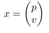
At each estimate, we associate a measure of uncertainty P. Using the uncertainty is great, because we can consider the fact that LiDARs are more accurate than RADARs in our measurements!
By performing a data fusion, we consider the sensor noise and outputs.
To give an example, look at this fusion of 2 LiDARs looking at a pedestrian.
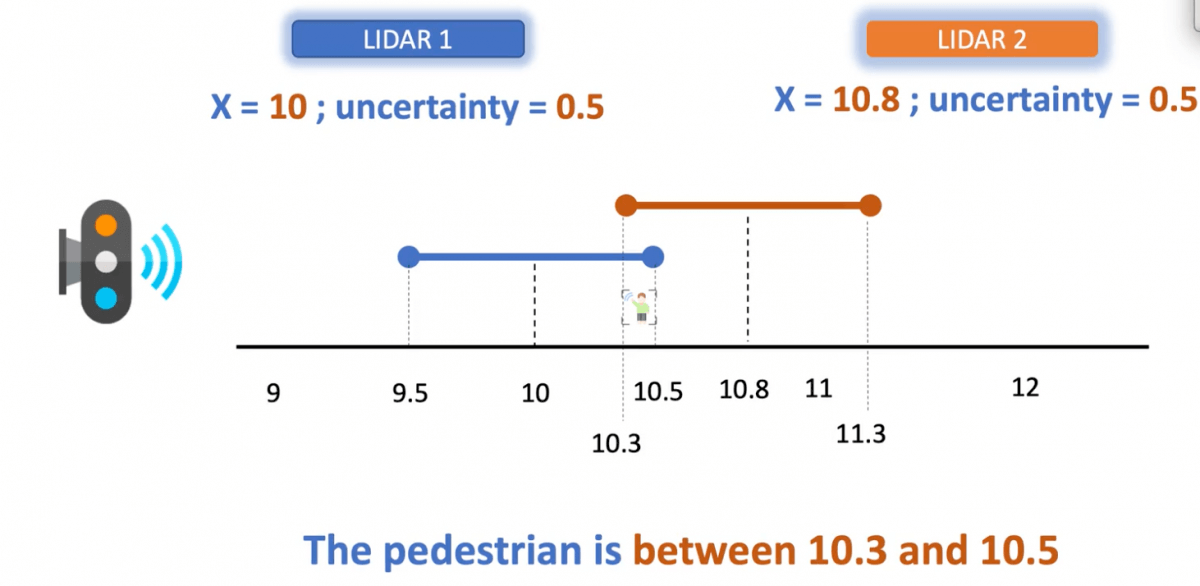
Both sensors are equally certain, but we can see how things would have changed if they weren't.
Considering multiple sensors and their uncertainties help us get a better idea of the pedestrian's position than if we had only one sensor.
Now, let's take a look at how we actually use Kalman Filters in RADAR/LIDAR fusion. To start, we'll need to understand the way sensor fusion algorithms such as Kalman Filters represent our estimates; using gaussians.
Gaussians
State and uncertainty are represented by Gaussians.
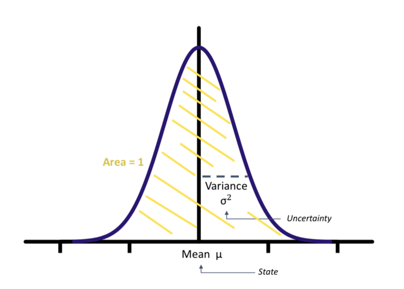
A Gaussian is a continuous function under which the area is 1. As you can see here, the gaussian is a formula that is centered around what we call the mean, and the covariance helps to understand how "certain" we are.
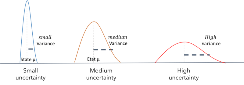
We have a mean μ representing a state and a variance σ² representing an uncertainty. The larger the variance, the greater the uncertainty.
Gaussians make it possible to estimate probabilities around the state and the uncertainty of a system.
We are on a probability to normal distribution. A Kalman Filter is unimodal: it means that we have a single peak each time to estimate the state of the system.
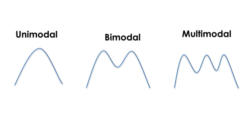
Put differently: the obstacle is not both 10 meters away with 90% and 8 meters away with 70%; it's 9.7 meters away with 98% or nothing.
A Kalman filter is a continuous and uni-modal function.
So far, we've seen how Kalman Filters help us in the representation process, but not in the sensor fusion process. Now, let's consider sensor fusion by understanding a key concept: Bayesian Filtering.
Bayesian Filtering
A Kalman filter is an implementation of a Bayesian filter, ie. alternating between prediction and update over and over again.
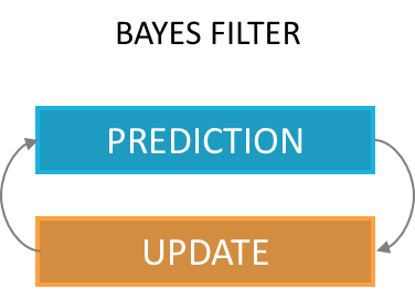
- Prediction : We use the estimated state to predict the future state and uncertainty.
- Update : We use the observations of our sensors to correct the prediction and obtain an even more accurate estimate.
Here's what sensor fusion can look like -- A sensor data arrives; we update the estimated position of the pedestrian we're tracking and predict its next one. Next -- Anew sensor data arrives, we update the position, and grade how well we manage to predict, and predict the next one considering that.
⚠️ To make an estimate a Kalman Filter, it only needs the current observations and the previous prediction. The measurement history is not necessary. It's not Machine Learning, it's Artificial Intelligence. This tool is therefore light and improves with time.
Let's take a step back and analyze everything we've learned so far:
- We are doing sensor fusion between LiDAR and RADAR
- But only their respective outputs (late fusion)
- For that, we're using a Kalman Fitler
- Which are unimodals and use Gaussians to represent state and uncertainty
- And work using a Prediction/Update Cycle, also called Bayesian Filtering.
Now, let's look at how it works under the hood.
The Maths behind Kalman Filters
The mathematics behind the Kalman filters are made of additions and multiplications of matrices. We have two stages: Prediction and Update.
In this section, I'll give an overview of the formulas behind Kalman Filters. If you'd like to go further and truly understand and master these, enroll in my course LEARN KALMAN FILTERS: The Hidden Algorithms that Silently powers the future . There, you will learn how Kalman Filters work, you will understand the maths, and code your own Kalman Filter from scratch for different use cases.
Prediction Formulas
Our prediction consists of estimating a state x’ and an uncertainty P’at time t+1 from the previous states x and P at time t.
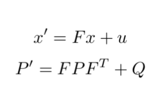
We therefore have just two formulas to estimate x and P. The other values are:
- F: Transition matrix from t to t+1
- ν: Noise
- Q: Covariance matrix including noise
👉 If we simplify things -- we can say that our new position x' is equal to the former position x, times a matrix F. This matrix F is called our motion model.
Here's a short example on what it looks like and how to use it.
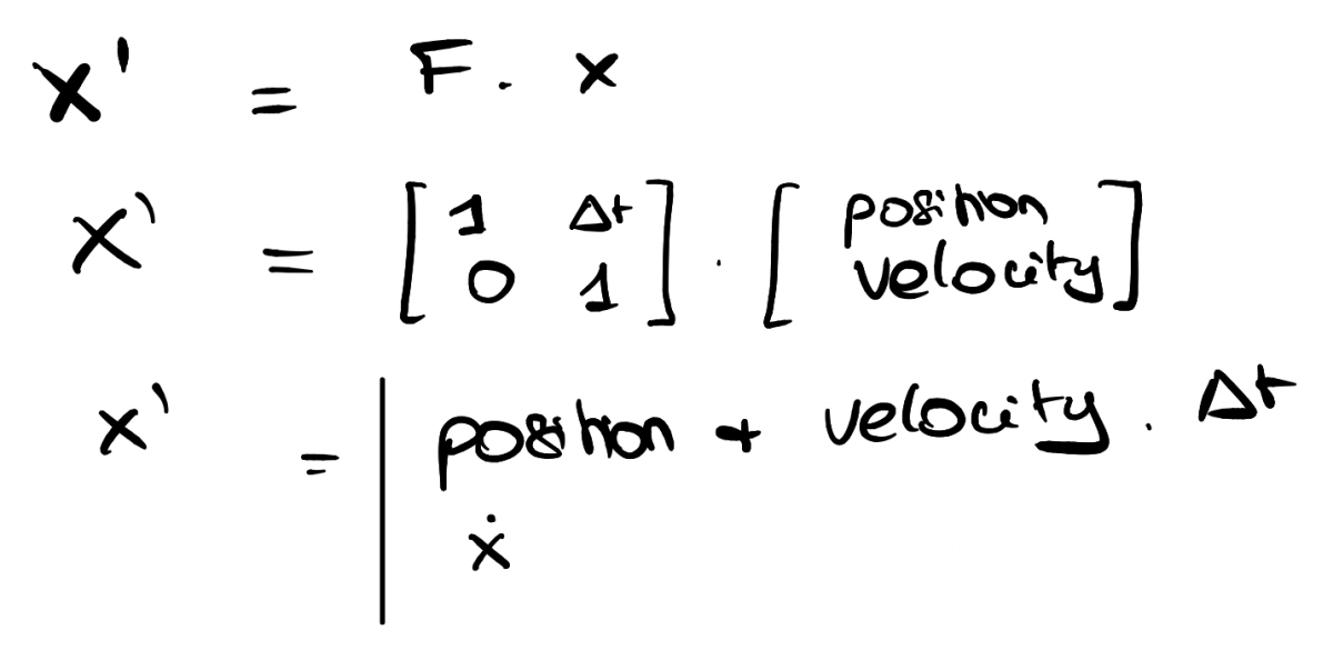
As you can see, F is simply a matrix describing how we move from step t to step t+1.
Here, we have:
- position (t+1) = position (t) + velocity (t)*time
- velocity (t+1) = velocity (t)
Put differently, we consider a constant velocity.
Our predict equations are meant to translate the movement between two time frames . We can make the F matrix implement different motion models such as Constant Turn Rate, Constant Velocity, Constant Acceleration, ...
So this is how we predict the next position - F is a matrix used to translate a movement. Now, let's look at the update formulas.
Update Formulas
In the update step, we want to adjust our position, and correct how we'll predict at the next step.

Let's take a look at how this works -- We have x' (predicted state) and P' (predicted covariance) for time t+1.
Now, we receive a new sensor data and can confirm if we were close or not.
- y is the difference between the actual measurement and our prediction -- it's the error in prediction!
- The other matrices are here to considersensor noise (R), estimate a system error (S), and a Kalman Gain (K) -- that last value is between 0 and 1 and helps decide if we should trust the prediction or the measurement more than the other.
- All of these leads to calculating a new x and a new P.
The update phase makes it possible to estimate an x and a P closer to reality than what the measurements and predictions provide.
After a few cycles, the Kalman Filter will converge, making more and more accurate predictions.
Before taking a look back and looking at the bigger picture, let's just consider the following about Bayesian Probabilities.
Prior/Posterior & Bayesian Filtering
This diagram show the ultimate maths inside a bayesian filter.
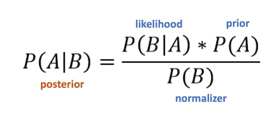
What we want to estimate is called the posterior. Mathematically, it's equal to the prior (prediction) times the likelihood (measurement).
The translation of that into gaussian is as follows:
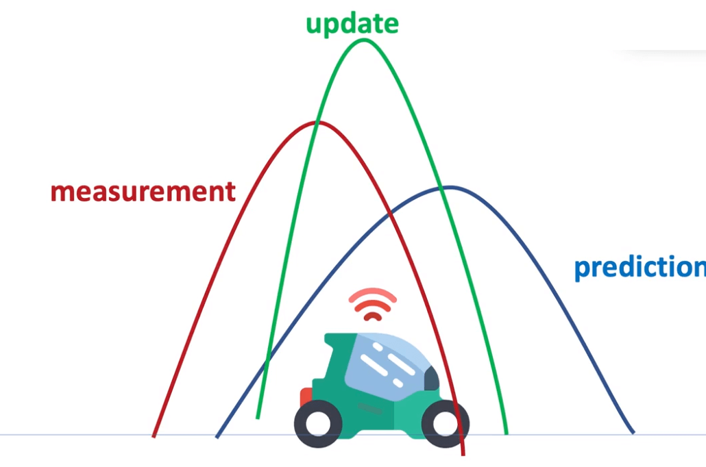
As you can see, the update (posterior) is always the best estimate. Then comes the measurement and the prediction, which is naturally the least certain of the 3.
At this point, you're probably thinking " Okay... that's cool, but Jeremy, you didn't talk about LiDARs and RADARs... You just talked about Sensor Fusion in a very general way. "
And you're right, so let's get to the meat.
RADAR/LiDAR Sensor Fusion Flow
The flow is as follows: each time a sensor comes, we're running a new Prediction+Update cycle.
Every prediction reduces the certainties, and every update increases it. But in the end, using both allows for more data, and for a better general result.
Something to understand: we're always working with the same values - our state (position, velocity) estimate.
Using Kalman Filters in RADAR LiDAR Fusion
When working with a LiDAR, we have "cartesian", linear values. Our mathematical formulas are all implemented with linear functions of type y = ax + b.
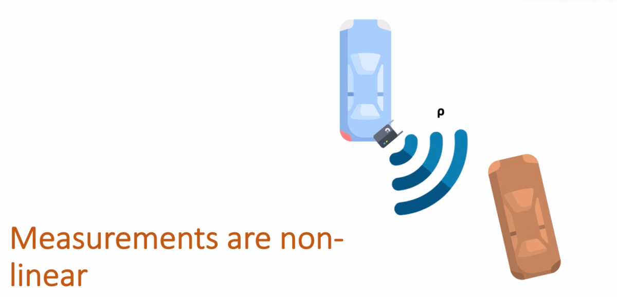
On the other hand, when we use a RADAR, the data is not linear. This sensor sees the world with three measures:
- 𝞺 (rho) : The distance to the object that is tracked.
- φ (phi) : The angle between the x-axis and our object.
- 𝞺 ̇ (rhodot) : The change of 𝞺, resulting in a radial velocity.
These three values make our measurement a nonlinear given the inclusion of the angle φ .
It means that when using RADARs, everything I just talked about it wrong and cannot work.
Non-Linear Kalman Filters
Everything here brings us to this point - The world is non-linear. Not everything moves perfectly in a straight line. Sensors don't all work the same way. For that reason, we must use two specific types of Kalman Filters:
- Extended Kalman Filters
- Unscented Kalman Filters
These filters will first "linearize" the non-linear data, so that it can work in a classic filter. In the extended version, we linearize the data using Jacobians and Taylor Series. In the Unscented Version, we use Sigma Point Prediction.
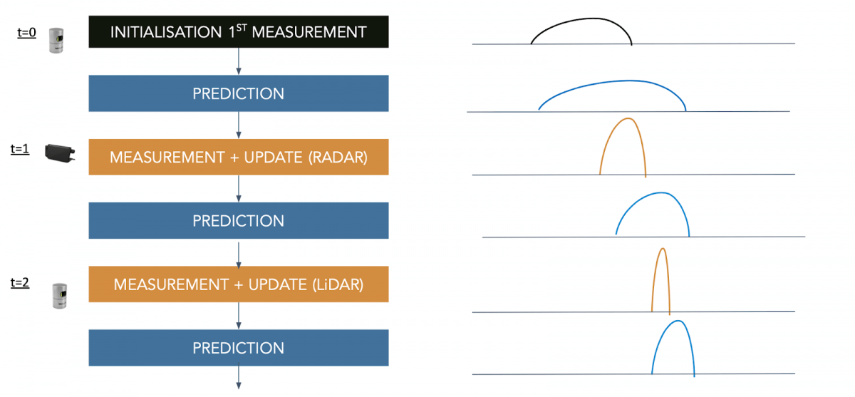
Final Sensor Fusion Flow
Considering this, here's our final sensor fusion flow.
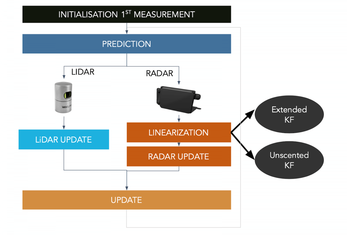
The LiDAR performs a regular update while the RADAR has to go through the linearization process. The cycle repeats itself again and again. We're never fusing the data together, it's always one after the other.
Results
The following videos present the results for an extended Kalman filter and an unscented kalman filter. We can see in particular oursensor (black origin), the Radar data (red), the Lidar data (blue) and our prediction (green). Each time we receive some data from one of our sensor, we realize a prediction.
Now, let's see the results using an Unscented Kalman Filter.

RMSE values are Root Mean Squared Error measures, which is the error between our prediction and the reality.
👉 The error is lower for the unscented filter than extended because this technique is more efficient.
We therefore have two techniques - one that seems better than the other for this specific use case.
Conclusion
Sensor fusion is one of the most important topics in a self-driving car. Sensor Fusion algorithms allow a vehicle to understand exactly how many obstacles there are, to estimate where they are and how fast they are moving. That's essential.
They always depend on the sensors that we have: Kalman Filters is not a systematic answer.
A final word - This skill is super hot to master. Using multiple sensors is now done on a daily basis. It's used in object detection, in localization, in positioning, in Computer Vision, in tracking.
To read more about Sensor Fusion -
I’ll see you tomorrow for your first email!