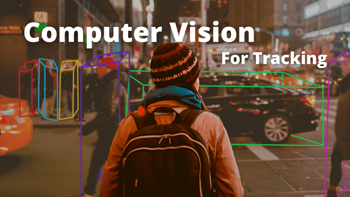
Computer Vision for Multi-Object Tracking — Live Example
In Computer Vision, one of the most interesting areas of research is obstacle detection using Deep Neural Networks. A lot of papers went out, all achieving SOTA (State of the Art) in detecting obstacles with a really high accuracy. The goal of these algorithms is to predict a list of bounding boxes from an input image. YOLO, SSD, RetinaNet, they are all faster and more accurate than the others in finding bounding boxes in real-time. In this article, I want to take a look at something called Multi-Object Tracking. How does Object Tracking work in Computer Vision?There are 3 ways to can track obstacles using Computer Vision.
- Feature Tracking — You can check my article Visual Features & Tracking that explains the fundamentals of the toic.
- Multi-Object Tracking — What we'll see in this article.
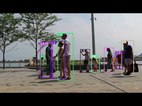
Let's take a look at why I think we should track bounding boxes... Here’s one of the most popular object detection algorithm, called YOLO (You Only Look Once).

2D Object Detection algorithms such as YOLO are very popular. In fact, they're the algorithms everybody wants to learn! Here's a video that explains the general idea. The question is, are they useful?
What this algorithm will output is a list of bounding boxes, in format [class, x, y, w, h, confidence]. The class is an id related to a number in a txt file (0 for car , 1 for pedestrian, …). x, y, w and h represent the parameters of the bounding box. x and y are the coordinates of the center while w and h are its size (width and height). The confidence is a score value expressed in %.
How can we use these bounding boxes ?
So far, bounding boxes have been used to count the number of obstacles of the same class in a crowd , in self-driving cars, drones, surveillance cameras, autonomous robots, and all sorts of systems using Computer Vision. However, they all share the same limit: same class obstacles are from the same color and cannot be set apart.
Enters Deep SORT.
Deep SORT (Deep Simple Online Realtime Tracking)
This implementation uses an object detection algorithm, such as YOLOv5 and a system to track obstacle. As you can see, it works with occlusion as well. How? We need 2 algorithms for that: the Hungarian algorithm, and the Kalman filter.
- The Hungarian algorithm can tell if an object in current frame is the same as the one in previous frame. It will be used for association and id attribution. I have an entire article on the topic here.
- The Kalman Filter is an algorithm that can predict future positions based on current position. It can also estimate current position better than what the sensor or algorithm is telling us. It will be used to have better association.
The Hungarian Algorithm (Kuhn-Munkres)
The Hungarian Algorithm, also known as Kuhn Munkres algorithm, can tell whether an obstacle from one frame is the same as another obstacle from another frame.
To understand how we'll do the association, let's consider the following example...
Association example
In this example, we have frames at time t0 and t1.
- At t0 (top left), we have 3 obstacles with id 1, 2, and 3.
- At t1 (bottom left), we also have 3 obstacles, but these are not the same:
- 1 and 2 have been detected again
- 3 from t0 has not been detected
- There is also a new obstacle
- After the association, we consider that:
- Obstacle with ID 3 is a memory obstacle (missed detection), and it will be remove if we don't see it again for x frames.
- Obstacle with ID 4 is a new obstacle, and it will be used right away with ID 4!
As you can see, we have a lot of freedom! We can decide that obstacle 4 must be matched for 2 seconds before being considered a true obstacle, and we'd avoid false positives! Or we could consider that obstacle 3 should be removed right away, because it hasn't been detected at time t1!
How to obstain something like this? Well, let's our example and use the Hungarian Algorithm!
- We have two lists of boxes from YOLO: a tracking list (t-1) and a detection list (t).
- We go through these 2 lists, and calculate a score on the bounding boxes; it can be an IOU score, a shape score, the convolutional score, ... It can even be a combination of all 3!
For this example, let’s consider the IOU (Intersection Over Union) of the bounding boxes. It's a score telling us how much the boxes overlap, the more overlap, the higher the IOU.
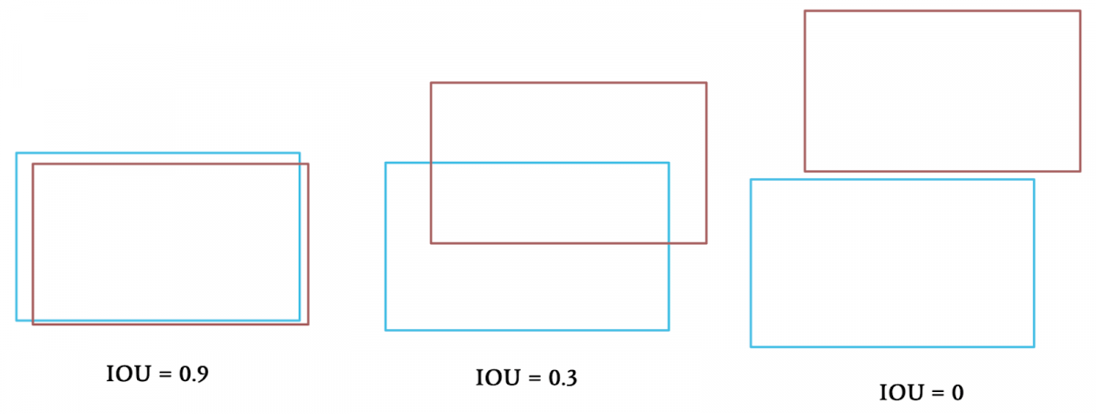
- In some cases, we have 20 boxes per image and some of them overlap. To solve this, we can take the argmax and set the maximum IOU value to 1 and all the others to 0.
Here's what our matrix looks like now, and let's remember that there is one detection that hasn't been matched, while there is an old track that hasn't been matched either.
- This is when we use the Hungarian Algorithm!
We have a matrix telling us the IOU scores between Detection and Trackings. By calling the sklearn function linear_assignment(), we are calling the optimization algorithm. This algorithm uses bipartite graph (graph theory) to find for each detection, the lowest tracking value in the matrix. Since we have scores and not costs, we will replace our 1 with -1; the minimum will be found. For our example, the hungarian matrix will be :
We can then check the values missing in our Hungarian Matrix and consider them as unmatched detections, or unmatched trackings. For detections, please consider A, B, C to have id 0,1,2.
For a deeper understanding of this article, check my article Inside the Hungarian Algorithm: A Self-Driving Car Example.
The next step of this algorithm is to use a Kalman Filter.
The Kalman Filter
Kalman Filters are very popular in most state estimation cases. It's been used to take Apollo XI to the moon, and it keeps being used in self-driving cars today, but also in robots, drones, self-flying planes, multi-sensor fusion, …→ For an understanding on how Kalman Filters work, I highly recommend my course LEARN KALMAN FILTERS: The Hidden Algorithm that Silently Powers the Future.
Here's why we're using a Kalman Filter: we have our bounding boxes on frame 1 and frame 2, but there is a motion between frame 1 and frame 2. The boxes moved, and if they moved too much, there is a risk of the IOU score being lower than it should and thus the match being lost. We're using Kalman Filters to predict the motion of the boxes between frame 1 and frame 2!
A Kalman Filter is used on every bounding box, so it comes after a box has been matched. When the association is made, predict and update functions are called. These functions implement the math of Kalman Filters composed of formulas for determining state mean and covariance.
Tracking Bounding Boxes with Mean and Covariance
Mean and Covariance are what we want to estimate. Mean is the coordinates of the bounding box, Covariance is our uncertainty on this bounding box having these coordinates.
- Mean (x) is a state vector. It is made of the coordinates of the center of the bounding box (cx,cy), size of the box (width, height) and the change of each of these parameters (velocities).
When we initialize this parameter, we set velocities to 0. They will then be estimated by the Kalman Filter.
- Covariance (P) is our uncertainty matrix in the estimation. We will set it to an arbitrary number and tweak it to see results. A larger number means a larger uncertainty.
That’s all we need to estimate: a state and an uncertainty!There is two steps for a Kalman Filter to work: prediction and update. Prediction will predict future positions, update will correct them and enhance the way we predict by changing the uncertainty. With time, a Kalman Filter gets better and better and converges to the optimal solution.
The Prediction/Update Cycle
Here's how it works in our example:
- At time t-1, we measure 3 bounding boxes. The Hungarian Algorithm defines them at 3 new detections. We therefore inialize a mean and a covariance with the values I showed before, for every bounding box.
- At time t=1, our detections become tracking, and we have 3 new detections! We start by calling the predict function to predict where the boxes from time t-1 will be at time t. Then, these predicted boxes are matched with the new boxes using the hungarian algorithm, and we call the update function to adjust our matrices and make a better prediction at the next timestep.
Prediction
Prediction phase is matrix multiplication that will tell us the position of our bounding box at time t based on its position at time t-1 .
So imagine we have a function called predict() in a class Kalman Filter that implements these maths. All we need to do is to have correct matrices F, Q and u. We will not use theu vector as it is used to estimate external forces, which we can’t really do easily here.
How to set up the matrices correctly ?
State Transition — F
F is the core implementation of the motion of our boxes from two timesteps. What we put here is important because when we will multiply x by F, we will change our x and have a new x, called x’.
As you can see, F [8x8] matrix contains a time value: dt is the difference between current frame and former frame timestamp. We will end up having cx’ = cx + dt*vx for the first line, cy’ = cy + dt*vy for the second, and so on…In this case, it means that we consider the velocity to be constant. We therefore set up F to implement the Constant Velocity model. There are a lot of models we can use depending on the problem we want to solve.
Process Covariance Matrix — Q
Q [8x8] is our noise matrix. It is how much confidence we give in the system. Its definition is very important and can change a lot of things. Q will be added to our covariance and will then define our global uncertainty. We can put very small values (0.01) and change it with time.Based on these matrices, and our measurement, we can now make a prediction that will give us x’ and P’. This can be used to predict future or actual positions. Having a matrix of confidence is useful for our filter that can model uncertainty of the world and of the algorithm to get better results.
Update
Update phase is a correction step. It includes the new measurement (z) and helps improve our filter.
The process of update is to start by measuring an error between measurement (z) and predicted mean. The second step is to calculate a Kalman Gain (K). The Kalman gain is used to estimate the importance of our error. We use it as a multiplication factor in the final formula to estimate a new x.
Again, How to set up the matrices correctly ?
Measurement Vector — Z
z is the measurement at time t. We don’t input velocities here as it is not measured, simply measured values.
Measurement Matrix — H
H [4x8] is our measurement matrix, it simply makes the math work between all or different matrices. We put the ones according to how we defined our state, and its dimension highly depends on how we define our state.
Measurement Noise — R
R is our measurement noise; it’s the noise from the sensor. For a LiDAR or RADAR, it’s usually given by the constructor. Here, we need to define a noise for YOLO algorithm, in terms of pixels. It will be arbitrary, we can say that the noise in terme of the center is about 1 or 2 pixels while the noise in the width and height can be bigger, let’s say 10 pixels.
Matrix multiplications are made; and we have a prediction and update loop that gets us better results than the yolo algorithm. The filter can also be used to predict at time t+1 (prediction with no update) from time t. For that, it needs to be good enough and have a low uncertainty.
Conclusion
We now understand how to track an obstacle through time:
- Detect obstacles bounding boxes.
- Match each box with the ones from t-1 using the Hungarian Algorithm. The cost metric can be IOU, or convolutional features (Deep SORT).
- Predict the next boxes using a Kalman Filter.
From there, we could use Machine Learning to predict future behavior or trajectories, we could be able to estimate what an obstacle will be doing the next 3 seconds. This tool is powerful and tracking become not only possible, but also very accurate. Velocities can be estimated and a huge set of possibilities becomes available.
In this article, we learned how to turn basic Object Detection skills, which today is common, into Object Tracking skills, which is valuable. Many of my clients learned to make their profile special using these skills that are valuable, but not found everywhere...
If you're interested in the topic, I have build a course called LEARN OBSTACLE TRACKING: The Master Key to become a Self-Driving Car Professional is my course on the implementation of Multi-Object Tracking for the Hungarian Algorithm. Inside, you'll:
- Understand how Multi-Object Tracking works and learn to become a Prediction Engineer
- Implement your own algorithms, and study each of them in-depth
- Build a cutting-edge project to track obstacles in Paris
- and much more...
You can visit the course here!